Thermal Distribution Functions

Introduction

In this notebook we wish to compute the thermal distribution functions for fermions and bosons. The functions we wish to compute are the equilibirium number, energy, pressure and entropy densities. In full form, these are given by: $$\begin{align} n(T) &= g\int\dfrac{d^3k}{(2\pi)^2}f(\mathbf{k})\\\ \rho(T) &= g\int\dfrac{d^3k}{(2\pi)^2}E(\mathbf{k})f(\mathbf{k})\\\ P(T) &= g\int\dfrac{d^3k}{(2\pi)^2}\dfrac{|\mathbf{k}|^2}{3E(\mathbf{k})}f(\mathbf{k}) \end{align}$$ with $g$ representing the number of internal degrees of freedom (d.o.f), $E^2 = k^2 + m^2$ and $f(\mathbf{k})$ is the phase-space distribution function. For a species in kinetic equilibirium, the phase space distribution is given by: $$\begin{align} f(\mathbf{k}) &= \dfrac{1}{e^{E/T}\pm1} \end{align}$$ where one takes the $+$ for fermions and $-$ for bosons. Note that we have ignored the chemical potential in writing down $f$. Since $f(\mathbf{k})$ is independent of angles, we can integrate of the solid angle and obtain: $$\begin{align} n(T) &= \dfrac{g}{2\pi^2}\int_{m}^{\infty} dE \dfrac{E\sqrt{E^2-m^2}}{e^{E/T}\pm1}\\ \rho(T) &= \dfrac{g}{2\pi^2}\int_{m}^{\infty} dE \dfrac{E^2\sqrt{E^2-m^2}}{e^{E/T}\pm1}\\ P(T) &= \dfrac{g}{6\pi^2}\int_{m}^{\infty} dE \dfrac{(E^2-m^2)^{3/2}}{e^{E/T}\pm1} \end{align}$$ We can further simplify these functions by defining: $z = E / T$ and $x = m / T$. Doing so, we find

$$\begin{align} n(T) &= gT^3\bar{n}_{\pm}(x)\\\ \rho(T) &= gT^4\bar{\rho}_{\pm}(x)\\\ P(T) &= gT^4\bar{P}_{\pm}(x) \end{align}$$

where we defined the ‘barred’ quantities as:

$$\begin{align} \bar{n}_{\pm}(x) &= \dfrac{1}{2\pi^2}\int_{x}^{\infty} dz \dfrac{z\sqrt{z^2-x^2}}{e^{z}\pm1}\\ \bar{\rho}_{\pm}(x) &= \dfrac{1}{2\pi^2}\int_{x}^{\infty} dz \dfrac{z^2\sqrt{z^2-x^2}}{e^{z}\pm1}\\ \bar{P}_{\pm}(x) &= \dfrac{1}{6\pi^2}\int_{x}^{\infty} dz \dfrac{(z^2-x^2)^{3/2}}{e^{z}\pm1} \end{align}$$

Let’s define functions for these quantities. We will negelect $g$ and factors of $T$ for now since they only contribute scaling.

using QuadGK

"""
  nbar(x, stats)

Integral representation of n̄

# Arguments
-`x::Float64`: mass of particle divided by temperature
-`stats::Symbol`: `:boson` or `:fermion`
"""
function nbar(x::Float64, stats::Symbol)
  pf::Float64 = 1 / (2π^2)
  function integrand(z::Float64)
    if stats == :boson
      return z * sqrt(z^2 - x^2) / (exp(z) - 1)
    elseif stats == :fermion
      return z * sqrt(z^2 - x^2) / (exp(z) + 1)
    else
      return 0.0
    end
  end
  return quadgk(integrand, x, Inf)[1] / (2π^2)
end

"""
  ρbar(x, stats)

Integral representation of ρ̄

# Arguments
-`x::Float64`: mass of particle divided by temperature
-`stats::Symbol`: `:boson` or `:fermion`
"""
function ρbar(x::Float64, stats::Symbol)
  function integrand(z::Float64)
    if stats == :boson
      return z^2 * sqrt(z^2 - x^2) / (exp(z) - 1)
    elseif stats == :fermion
      return z^2 * sqrt(z^2 - x^2) / (exp(z) + 1)
    else
      return 0.0
    end
  end
  return quadgk(integrand, x, Inf)[1] / (2π^2)
end

"""
  pbar(x, stats)

Integral representation of p̄

# Arguments
-`x::Float64`: mass of particle divided by temperature
-`stats::Symbol`: `:boson` or `:fermion`
"""
function pbar(x::Float64, stats::Symbol)
  function integrand(z::Float64)
    if stats == :boson
      return (z^2 - x^2)^1.5 / (exp(z) - 1)
    elseif stats == :fermion
      return (z^2 - x^2)^1.5 / (exp(z) + 1)
    else
      return 0.0
    end
  end
  return quadgk(integrand, x, Inf)[1] / (6π^2)
end;

Let’s plot the results of these functions:

import PyPlot; const plt = PyPlot # python plotting
using LaTeXStrings

xs = 10 .^(range(-1, stop=1, length=100))
nbar_fermions = [nbar(x, :fermion) for x in xs]
ρbar_fermions = [ρbar(x, :fermion) for x in xs]
pbar_fermions = [pbar(x, :fermion) for x in xs]

nbar_bosons = [nbar(x, :boson) for x in xs]
ρbar_bosons = [ρbar(x, :boson) for x in xs]
pbar_bosons = [pbar(x, :boson) for x in xs]

plt.figure(dpi=100)
plt.plot(xs, nbar_fermions, label=L"$\bar{n}$ fermions")
plt.plot(xs, ρbar_fermions, label=L"$\bar{\rho}$ fermions")
plt.plot(xs, pbar_fermions, label=L"$\bar{P}$ fermions")

plt.plot(xs, nbar_bosons, "--", label=L"$\bar{n}$ bosons")
plt.plot(xs, ρbar_bosons, "--", label=L"$\bar{\rho}$ bosons")
plt.plot(xs, pbar_bosons, "--", label=L"$\bar{P}$ bosons")

plt.yscale("log")
plt.xscale("log")
plt.xlabel(L"$x$", fontsize=16)
plt.ylim([1e-3, 1])
plt.xlim([1e-1, 1e1])
plt.legend()
plt.gcf()

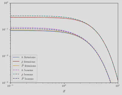
There are a few things to take away from this plot. The first is that the asymptotic behaviour as $x\to\infty$ is independent of statistics. The reseason for this is clear: as $x\to\infty$, the integrand starts off with a very large value of $z$ and hence, $e^{z} \gg \pm1$. The second thing to notice is that the asymptotic behavior of $\bar{n}$ and $\bar{P}$ are identical, but they differer from the asymptotic behavior of $\bar{\rho}$. The third thing to notice is that the differences between fermions and bosons is small. We will show why that’s the case later on.

Asymptotic forms

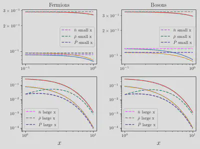
The integrals for the number, energy and pressure densities can be evaluated exactly for $x\ll 1$ and $x\gg1$. If we set $x = 0$, then the results are:

$$ \begin{align} \bar{n}(x) &= \dfrac{\zeta(3)}{\pi^2} \begin{cases} 1 & \text{bosons}\\ 3/4 & \text{fermions} \end{cases}\\ \bar{\rho}_{\pm}(x) &= \dfrac{\pi^2}{30} \begin{cases} 1 & \text{bosons}\\ 7/8 & \text{fermions} \end{cases}\\ \bar{P}_{\pm}(x) &= \bar{\rho}/3 \end{align} $$

In the opposite limit, we can simply ignore the statistics factors in the denominators of the integral, obtaining:

$$ \begin{align} \bar{n}(x) &= e^{-x}\left(\frac{x}{2\pi}\right)^{3/2}\\ \bar{\rho}_{\pm}(x) &= xe^{-x}\left(\frac{x}{2\pi}\right)^{3/2}\\ \bar{P}_{\pm}(x) &= e^{-x}\left(\frac{x}{2\pi}\right)^{3/2}\\ \end{align} $$

Let’s check that these are correct:

using SpecialFunctions
nbar_small_x_b = zeta(3)/π^2
nbar_small_x_f = 3/4 * zeta(3)/π^2
ρbar_small_x_b = π^2/30
ρbar_small_x_f = 7/8 * π^2/30
pbar_small_x_b = π^2/90
pbar_small_x_f = 7/8 * π^2/90

nbar_large_x(x::Float64) = exp(-x) * (x/(2π))^1.5
ρbar_large_x(x::Float64) = x * exp(-x) * (x/(2π))^1.5
pbar_large_x(x::Float64) = exp(-x) * (x/(2π))^1.5

xs = 10 .^(range(-1, stop=0, length=100))
nbar_fermions = [nbar(x, :fermion) for x in xs]
ρbar_fermions = [ρbar(x, :fermion) for x in xs]
pbar_fermions = [pbar(x, :fermion) for x in xs]

nbar_bosons = [nbar(x, :boson) for x in xs]
ρbar_bosons = [ρbar(x, :boson) for x in xs]
pbar_bosons = [pbar(x, :boson) for x in xs]

plt.figure(dpi=100)
plt.subplot(2, 2, 1)
plt.title("Fermions")
plt.plot(xs, nbar_fermions)
plt.plot(xs, ρbar_fermions)
plt.plot(xs, pbar_fermions)

plt.plot(xs, [nbar_small_x_f for _ in xs], "--", label=L"$\bar{n}$ small x")
plt.plot(xs, [ρbar_small_x_f for _ in xs], "--", label=L"$\bar{\rho}$ small x")
plt.plot(xs, [pbar_small_x_f for _ in xs], "--", label=L"$\bar{P}$ small x")
plt.yscale("log")
plt.xscale("log")
plt.legend()

plt.subplot(2, 2, 2)
plt.title("Bosons")
plt.plot(xs, nbar_bosons)
plt.plot(xs, ρbar_bosons)
plt.plot(xs, pbar_bosons)
plt.plot(xs, [nbar_small_x_b for _ in xs], "--", label=L"$\bar{n}$ small x")
plt.plot(xs, [ρbar_small_x_b for _ in xs], "--", label=L"$\bar{\rho}$ small x")
plt.plot(xs, [pbar_small_x_b for _ in xs], "--", label=L"$\bar{P}$ small x")
plt.yscale("log")
plt.xscale("log")
plt.legend()

xs = 10 .^(range(0, stop=1, length=100))
nbar_fermions = [nbar(x, :fermion) for x in xs]
ρbar_fermions = [ρbar(x, :fermion) for x in xs]
pbar_fermions = [pbar(x, :fermion) for x in xs]

nbar_bosons = [nbar(x, :boson) for x in xs]
ρbar_bosons = [ρbar(x, :boson) for x in xs]
pbar_bosons = [pbar(x, :boson) for x in xs]

plt.subplot(2, 2, 3)
plt.plot(xs, nbar_fermions)
plt.plot(xs, ρbar_fermions)
plt.plot(xs, pbar_fermions)
plt.plot(xs, [nbar_large_x(x) for x in xs], "--", label=L"$\bar{n}$ large x")
plt.plot(xs, [ρbar_large_x(x) for x in xs], "--", label=L"$\bar{\rho}$ large x")
plt.plot(xs, [pbar_large_x(x) for x in xs], "--", label=L"$\bar{P}$ large x")
plt.yscale("log")
plt.xscale("log")
plt.xlabel(L"$x$", fontsize=16)
plt.legend()

plt.subplot(2, 2, 4)
plt.plot(xs, nbar_bosons)
plt.plot(xs, ρbar_bosons)
plt.plot(xs, pbar_bosons)
plt.plot(xs, [nbar_large_x(x) for x in xs], "--", label=L"$\bar{n}$ large x")
plt.plot(xs, [ρbar_large_x(x) for x in xs], "--", label=L"$\bar{\rho}$ large x")
plt.plot(xs, [pbar_large_x(x) for x in xs], "--", label=L"$\bar{P}$ large x")
plt.yscale("log")
plt.xscale("log")
plt.xlabel(L"$x$", fontsize=16)
plt.legend()

plt.tight_layout()
plt.gcf()

Bessel Function Series of Thermal Functions

The integrals for $\bar{n}(x), \bar{\rho}(x)$ and $\bar{P}(x)$ can be evaluated exactly if one ignores the $\pm1$ in the denomiator of the integrands. This suggests that one may be able to perform a series expansion of the denominator in powers of $e^{-z}$ and evaluate the integrals exactly. This turns our to be true. Note that:

$$\begin{align} \dfrac{1}{e^{z}\pm1} &= \sum_{n=1}^{\infty}(\mp1)^{n+1}e^{-nz} \end{align}$$

Therefore, the functions $\bar{n}(x), \bar{\rho}(x)$ and $\bar{P}(x)$ can be written as:

$$ \begin{align} \bar{n}_{\pm}(x) &= \dfrac{1}{2\pi^2}\sum_{n=1}^{\infty}(\mp1)^{n+1}\int_{x}^{\infty} dz e^{-nz}z\sqrt{z^2-x^2}\\ \bar{\rho}_{\pm}(x) &= \dfrac{1}{2\pi^2}\sum_{n=1}^{\infty}(\mp1)^{n+1}\int_{x}^{\infty} dz e^{-nz}z^2\sqrt{z^2-x^2}\\ \bar{P}_{\pm}(x) &= \dfrac{1}{6\pi^2}\sum_{n=1}^{\infty}(\mp1)^{n+1}\int_{x}^{\infty} dz e^{-nz}(z^2-x^2)^{3/2} \end{align} $$

These integrals can be represented as modified bessel functions of the second kind:

$$ \begin{align} \bar{n}_{\pm}(x) &= \dfrac{x^2}{2\pi^2}\sum_{n=1}^{\infty}\dfrac{(\mp 1)^{n+1}}{n}K_{2}(nx)\\\ \bar{\rho}_{\pm}(x) &= \dfrac{x^2}{2\pi^2}\sum_{n=1}^{\infty}\frac{(\mp 1)^{n+1}}{n^2}\left[n x K_{1}(nx)+3K_{2}(nx)\right]\\ \bar{P}_{\pm}(x) &= \dfrac{x^2}{2\pi^2}\sum_{n=1}^{\infty}\frac{(\mp 1)^{n+1}}{n^2}K_{2}(nx) \end{align} $$

Let’s make functions for these sums:

using SpecialFunctions

"""
  nbar_bessel(x, stats, order)

Sum-of-bessel function representation of n̄

# Arguments
-`x::Float64`: mass of particle divided by temperature
-`stats::Symbol`: `:boson` or `:fermion`
-`order::Int64`: number of terms in series to keep
"""
function nbar_bessel(x::Float64, stats::Symbol, order::Int64)
  bsum::Float64 = 0.0
  if stats == :fermion
    bsum = sum([(-1)^(n+1) / n * besselk(2, n*x) for n in 1:order])
  elseif stats == :boson
    bsum = sum([1 / n * besselk(2, n*x) for n in 1:order])
  end
  bsum * x^2 / (2π^2)
end

"""
  ρbar_bessel(x, stats, order)

Sum-of-bessel function representation of ρ̄

# Arguments
-`x::Float64`: mass of particle divided by temperature
-`stats::Symbol`: `:boson` or `:fermion`
-`order::Int64`: number of terms in series to keep
"""
function ρbar_bessel(x::Float64, stats::Symbol, order::Int64)
  bsum::Float64 = 0.0
  if stats == :fermion
    bsum = sum([(-1)^(n+1) / n^2 * (n * x * besselk(1, n*x) +
                3 * besselk(2, n*x)) for n in 1:order])
  elseif stats == :boson
    bsum = sum([1 / n^2 * (n * x * besselk(1, n*x) +
                3 * besselk(2, n*x)) for n in 1:order])
  end
  bsum * x^2 / (2π^2)
end

"""
  pbar_bessel(x, stats, order)

Sum-of-bessel function representation of p̄

# Arguments
-`x::Float64`: mass of particle divided by temperature
-`stats::Symbol`: `:boson` or `:fermion`
-`order::Int64`: number of terms in series to keep
"""
function pbar_bessel(x::Float64, stats::Symbol, order::Int64)
  bsum::Float64 = 0.0
  if stats == :fermion
    bsum = sum([(-1)^(n+1) / n^2 * besselk(2, n*x) for n in 1:order])
  elseif stats == :boson
    bsum = sum([1 / n^2 * besselk(2, n*x) for n in 1:order])
  end
  bsum * x^2 / (2π^2)
end;

Let’s plot these functions and see that they are correct:

xs = 10 .^(range(-1, stop=log10(3), length=100))

nrows = 2
ncols = 3

plt.figure(dpi=100)
for nrow in 1:nrows
  stats = (nrow == 1) ? :boson : :fermion
  for ncol in 1:ncols
    plt.subplot(nrows, ncols, ncols * (nrow - 1) + ncol)
    if ncol == 1
      plt.title(L"$\bar{n}$ " * string(stats))
      exact = [nbar(x, stats) for x in xs]
      approx1 = [nbar_bessel(x, stats, 1) for x in xs]
      approx5 = [nbar_bessel(x, stats, 5) for x in xs]
    elseif ncol == 2
      plt.title(L"$\bar{p}$ " * string(stats))
      exact = [pbar(x, stats) for x in xs]
      approx1 = [pbar_bessel(x, stats, 1) for x in xs]
      approx5 = [pbar_bessel(x, stats, 5) for x in xs]
    elseif ncol == 3
      plt.title(L"$\bar{\rho}$ " * string(stats))
      exact = [ρbar(x, stats) for x in xs]
      approx1 = [ρbar_bessel(x, stats, 1) for x in xs]
      approx5 = [ρbar_bessel(x, stats, 5) for x in xs]
    end
    plt.plot(xs, exact, lw=3, alpha=0.6, label="exact")
    plt.plot(xs, approx1, "r--", label="n=1")
    plt.plot(xs, approx5, "k--", label="n=1:5")
    plt.yscale("log")
    plt.xscale("log")
    plt.xlim([minimum(xs), maximum(xs)])
    if ncol == 3 && nrow == 2
      plt.legend()
    end
  end
end

plt.tight_layout()
plt.gcf()

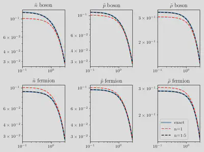
From these plots, we can see that even just the first term approximates the thermal functions quite well. In practice, it is a good approximation to take:

$$ \begin{align} \bar{n}_{\pm}(x) &= \dfrac{x^2}{2\pi^2}K_{2}(x)\\\ \bar{\rho}_{\pm}(x) &= \dfrac{x^2}{2\pi^2}\left[xK_{1}(x)+3K_{2}(x)\right]\\ \bar{P}_{\pm}(x) &= \dfrac{x^2}{2\pi^2}K_{2}(x) \end{align} $$

These approximations have the added benifit of being independent of statistics. The corrections for statistics come in when we include the second terms in the sums. Let’s plot the percent errors when only including the first and second terms in the series:

xs = 10 .^(range(-1, stop=log10(3), length=100))

nrows = 2
ncols = 3

plt.figure(dpi=100)
for nrow in 1:nrows
  stats = (nrow == 1) ? :boson : :fermion
  for ncol in 1:ncols
    plt.subplot(nrows, ncols, ncols * (nrow - 1) + ncol)
    if ncol == 1
      plt.title(L"$\bar{n}$ " * string(stats))
      exact = [nbar(x, stats) for x in xs]
      approx1 = [nbar_bessel(x, stats, 1) for x in xs]
      approx2 = [nbar_bessel(x, stats, 2) for x in xs]
      approx3 = [nbar_bessel(x, stats, 3) for x in xs]
    elseif ncol == 2
      plt.title(L"$\bar{p}$ " * string(stats))
      exact = [pbar(x, stats) for x in xs]
      approx1 = [pbar_bessel(x, stats, 1) for x in xs]
      approx2 = [pbar_bessel(x, stats, 2) for x in xs]
      approx3 = [pbar_bessel(x, stats, 3) for x in xs]
    elseif ncol == 3
      plt.title(L"$\bar{\rho}$ " * string(stats))
      exact = [ρbar(x, stats) for x in xs]
      approx1 = [ρbar_bessel(x, stats, 1) for x in xs]
      approx2 = [ρbar_bessel(x, stats, 2) for x in xs]
      approx3 = [ρbar_bessel(x, stats, 3) for x in xs]
    end
    if ncol == 1
      plt.ylabel(L"$\%$ error")
    end
    plt.plot(xs, abs.(exact .- approx1) ./ exact .* 100, label="n=1")
    plt.plot(xs, abs.(exact .- approx2) ./ exact .* 100, label="n=1:2")
    plt.plot(xs, abs.(exact .- approx3) ./ exact .* 100, label="n=1:3")
    plt.xscale("log")
    #plt.yscale("log")
    plt.xlim([minimum(xs), maximum(xs)])
    plt.ylim([0, 20])
    if ncol == 1 && nrow == 2
      plt.legend()
    end
  end
end

plt.tight_layout()
plt.gcf()

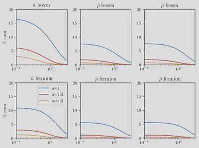
From these plots, we can see that we are always within 20% of the actual value even when only including the first term in the series. We see rapid global convergence when we begin including higher order terms.

Entropy Density

In addition to the number, pressure and energy density, one also typical cares about the entropy density. It can be shown that the entropy density is given by: $$\begin{align} s(T) &= \dfrac{\rho(T) + P(T)}{T} = gT^3(\bar{\rho}(x) + \bar{P}(x)) \end{align}$$ In integral form, this is: $$\begin{align} s(T) &= gT^3\bar{s}(x) \end{align}$$ where

$$ \begin{align} \bar{s}(x) &= \bar{\rho}(x) + \bar{P}(x) = \dfrac{1}{6\pi^2}\int_{x}^{\infty} dz \dfrac{(4z^2-x^2)\sqrt{z^2-x^2}}{e^{z}\pm1}\ \end{align} $$

In terms of bessel functions, this is:

$$ \begin{align} \bar{s}(x) &= \dfrac{x^3}{2\pi^2}\sum_{n=1}^{\infty}\dfrac{(\mp1)^{n+1}}{n}K_{3}(nx) \end{align} $$

Degrees of Freedom Stored in Energy and Entropy

When dealing with many species of particles, it is often useful to define the energy and entropy density in terms of a single function:

$$ \begin{align} \rho(T) &= \sum_{i}\rho_{i}(T) = T^4\sum_{i}g_{i}\bar{\rho}_{i}(x) \equiv \dfrac{\pi^2}{30}g_{\mathrm{eff}}(T)T^4\\ s(T) &= \sum_{i}s_{i}(T) = T^3\sum_{i}g_{i}\bar{s}_{i}(x) \equiv \dfrac{2\pi^2}{45}h_{\mathrm{eff}}(T)T^3 \end{align} $$

where the sum runs over all particles and the effective number of relativistic d.o.f. stored in energy and entropy $g_{\mathrm{eff}}$, $h_{\mathrm{eff}}$ are:

$$ \begin{align} g_{\mathrm{eff}}(T) &= \dfrac{30}{\pi^2}\sum_{i}g_{i}\bar{\rho}_{i}(x)\\\ h_{\mathrm{eff}}(T) &= \dfrac{45}{2\pi^2}\sum_{i}g_{i}\bar{s}_{i}(x) \end{align} $$

Derivatives of Thermal Functions

Lastly, let’s investigate the derivatives of the various functions. The derivatives are: $$\begin{align} \dfrac{dn}{dT} &= gT^2\left(3T\bar{n}(x)-x\dfrac{d\bar{n}}{dx}\right)\\\ \dfrac{d\rho}{dT} &= gT^3\left(4T\bar{\rho}(x)-x\dfrac{d\bar{\rho}}{dx}\right)\\\ \dfrac{dP}{dT} &= gT^3\left(4T\bar{P}(x)-x\dfrac{d\bar{P}}{dx}\right)\\\ \dfrac{ds}{dT} &= gT^2\left(3T\bar{s}(x)-x\dfrac{d\bar{s}}{dx}\right) \end{align}$$

We will want to compute derivatives of the barred quantities. All of the barred quantities are of the form: $$\begin{align} \int_{x}^{\infty}f(x,z)dz \end{align}$$ Using Leibniz’s rule for differentiating integrals, one finds that: $$\begin{align} \dfrac{d}{dx}\int_{x}^{\infty}f(x,z)dz = \int_{x}^{\infty}\dfrac{\partial f}{\partial x}dz - f(x, x) \end{align}$$ Notice that all the integrand for our function evaluated at $z=x$ are zero. Thus, we only need the integrate the derivative of the integrand w.r.t $x$. The derivatives are: $$\begin{align} \dfrac{d\bar{n}}{dx} &= -\dfrac{x}{2\pi^2}\int_{x}^{\infty}\dfrac{z}{(e^{z}-1)\sqrt{z^2-x^2}}\\ \dfrac{d\bar{\rho}}{dx} &= -\dfrac{x}{2\pi^2}\int_{x}^{\infty}\dfrac{z^2}{(e^{z}-1)\sqrt{z^2-x^2}}\\ \dfrac{d\bar{P}}{dx} &= -\dfrac{x}{2\pi^2}\int_{x}^{\infty}\dfrac{\sqrt{z^2-x^2}}{(e^{z}-1)} \end{align}$$ Let’s make some function for these and then invesigate how the look

"""
  nbar_deriv(x, stats)

Derivative of the integral representation of n̄

# Arguments
-`x::Float64`: mass of particle divided by temperature
-`stats::Symbol`: `:boson` or `:fermion`
"""
function nbar_deriv(x::Float64, stats::Symbol)
  pf::Float64 = 1 / (2π^2)
  function integrand(z::Float64)
    if stats == :boson
      return z / (exp(z) - 1) / sqrt(z^2 - x^2)
    elseif stats == :fermion
      return z / (exp(z) + 1) / sqrt(z^2 - x^2)
    else
      return 0.0
    end
  end
  return -x * quadgk(integrand, x, Inf)[1] / (2π^2)
end

"""
  ρbar_deriv(x, stats)

Derivative of the integral representation of ρ̄

# Arguments
-`x::Float64`: mass of particle divided by temperature
-`stats::Symbol`: `:boson` or `:fermion`
"""
function ρbar_deriv(x::Float64, stats::Symbol)
  function integrand(z::Float64)
    if stats == :boson
      return z^2 / (exp(z) - 1) / sqrt(z^2 - x^2)
    elseif stats == :fermion
      return z^2 / (exp(z) + 1) / sqrt(z^2 - x^2)
    else
      return 0.0
    end
  end
  return -x * quadgk(integrand, x, Inf)[1] / (2π^2)
end

"""
  pbar_deriv(x, stats)

Derivative of the integral representation of p̄

# Arguments
-`x::Float64`: mass of particle divided by temperature
-`stats::Symbol`: `:boson` or `:fermion`
"""
function pbar_deriv(x::Float64, stats::Symbol)
  function integrand(z::Float64)
    if stats == :boson
      return sqrt(z^2 - x^2) / (exp(z) - 1)
    elseif stats == :fermion
      return sqrt(z^2 - x^2) / (exp(z) + 1)
    else
      return 0.0
    end
  end
  return -x * quadgk(integrand, x, Inf)[1] / (2π^2)
end;

Now let’s plot:

xs = 10 .^(range(-1, stop=1, length=100))
nbar_deriv_fermions = [nbar_deriv(x, :fermion) for x in xs]
ρbar_deriv_fermions = [ρbar_deriv(x, :fermion) for x in xs]
pbar_deriv_fermions = [pbar_deriv(x, :fermion) for x in xs]

nbar_deriv_bosons = [nbar_deriv(x, :boson) for x in xs]
ρbar_deriv_bosons = [ρbar_deriv(x, :boson) for x in xs]
pbar_deriv_bosons = [pbar_deriv(x, :boson) for x in xs]

plt.figure(dpi=100)
plt.plot(xs, nbar_deriv_fermions, label=L"$d\bar{n}/dx$ fermions")
plt.plot(xs, ρbar_deriv_fermions, label=L"$d\bar{\rho}/dx$ fermions")
plt.plot(xs, pbar_deriv_fermions, label=L"$d\bar{P}/dx$ fermions")

plt.plot(xs, nbar_deriv_bosons, "--", label=L"$d\bar{n}/dx$ bosons")
plt.plot(xs, ρbar_deriv_bosons, "--", label=L"$d\bar{\rho}/dx$ bosons")
plt.plot(xs, pbar_deriv_bosons, "--", label=L"$d\bar{P}/dx$ bosons")

#plt.yscale("log")
plt.xscale("log")
plt.xlabel(L"$x$", fontsize=16)
#plt.ylim([1e-3, 1])
plt.xlim([minimum(xs), maximum(xs)])
plt.legend()
plt.gcf()

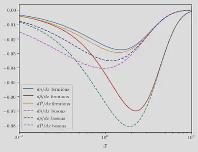
Next, let’s investigate the sum-over-bessel function representation of the derivatives. These are:

$$\begin{align} \bar{n}_{\pm}(x) &= -\dfrac{x^2}{2\pi^2}\sum_{n=1}^{\infty}(\mp1)^{n+1}K_{1}(nx)\\\ \bar{\rho}_{\pm}(x) &= -\dfrac{x^2}{2\pi^2}\sum_{n=1}^{\infty}\frac{(\mp1)^{n+1}}{n}\left[nxK_{0}(nx)+K_{1}(nx)\right]\\ \bar{P}_{\pm}(x) &= -\dfrac{x^2}{2\pi^2}\sum_{n=1}^{\infty}\frac{(\mp1)^{n+1}}{n}K_{1}(nx) \end{align}$$

Let’s make functions for these:

using SpecialFunctions

function nbar_deriv_bessel(x::Float64, stats::Symbol, order::Int64)
  bsum::Float64 = 0.0
  if stats == :fermion
    bsum = sum([(-1)^(n+1) * besselk(1, n*x) for n in 1:order])
  elseif stats == :boson
    bsum = sum([besselk(1, n*x) for n in 1:order])
  end
  -bsum * x^2 / (2π^2)
end

function ρbar_deriv_bessel(x::Float64, stats::Symbol, order::Int64)
  bsum::Float64 = 0.0
  if stats == :fermion
    bsum = sum([(-1)^(n+1) / n * (n * x * besselk(0, n*x) +
                besselk(1, n*x)) for n in 1:order])
  elseif stats == :boson
    bsum = sum([1 / n * (n * x * besselk(0, n*x) +
                besselk(1, n*x)) for n in 1:order])
  end
  -bsum * x^2 / (2π^2)
end

function pbar_deriv_bessel(x::Float64, stats::Symbol, order::Int64)
  bsum::Float64 = 0.0
  if stats == :fermion
    bsum = sum([(-1)^(n+1) / n * besselk(1, n*x) for n in 1:order])
  elseif stats == :boson
    bsum = sum([1 / n * besselk(1, n*x) for n in 1:order])
  end
  -bsum * x^2 / (2π^2)
end;

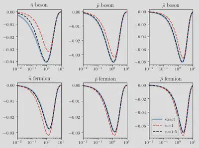
Now let’s plot to compare:

xs = 10 .^(range(-2, stop=1, length=100))

nrows = 2
ncols = 3

plt.figure(dpi=100)
for nrow in 1:nrows
  stats = (nrow == 1) ? :boson : :fermion
  for ncol in 1:ncols
    plt.subplot(nrows, ncols, ncols * (nrow - 1) + ncol)
    if ncol == 1
      plt.title(L"$\bar{n}$ " * string(stats))
      exact = [nbar_deriv(x, stats) for x in xs]
      approx1 = [nbar_deriv_bessel(x, stats, 1) for x in xs]
      approx5 = [nbar_deriv_bessel(x, stats, 5) for x in xs]
    elseif ncol == 2
      plt.title(L"$\bar{p}$ " * string(stats))
      exact = [pbar_deriv(x, stats) for x in xs]
      approx1 = [pbar_deriv_bessel(x, stats, 1) for x in xs]
      approx5 = [pbar_deriv_bessel(x, stats, 5) for x in xs]
    elseif ncol == 3
      plt.title(L"$\bar{\rho}$ " * string(stats))
      exact = [ρbar_deriv(x, stats) for x in xs]
      approx1 = [ρbar_deriv_bessel(x, stats, 1) for x in xs]
      approx5 = [ρbar_deriv_bessel(x, stats, 5) for x in xs]
    end
    plt.plot(xs, exact, lw=3, alpha=0.6, label="exact")
    plt.plot(xs, approx1, "r--", label="n=1")
    plt.plot(xs, approx5, "k--", label="n=1:5")
    #plt.yscale("log")
    plt.xscale("log")
    plt.xlim([minimum(xs), maximum(xs)])
    if ncol == 3 && nrow == 2
      plt.legend()
    end
  end
end

plt.tight_layout()
plt.gcf()