Temperature Evolution of a Decoupled Dark Sector
Introduction
In this document, we will invesigate how to compute the temperature and evolution of temperature of a species which is decoupled from the standard model. For simplicity, we will consider a set of particles which are decoupled from the standard model but are coupled in their own sector. If a species or set of species is completely decoupled from the standard model, then there should be no entropy exchange between the standard model and the secluded sector. Let’s denote the secluded sector as the “dark” sector. Then, the entropy density of the dark sector, denoted by $s_{d}$, is conserved in totality, i.e., $\frac{d}{dt}(a^3s_{d}) = 0$ ($a$ is the scale factor of the universe.) This implies that the ratio of entropy densities of the dark and standar model is a constant: $$\begin{align} \mathrm{constant} = \dfrac{a^3s_{d}(T_{d})}{a^3s(T)} = \dfrac{s_{d}(T_{d})}{s(T)} \end{align}$$ where $s$ is the standard model entropy density, $T_{d}$ is the dark sector temperature and $T$ is the standard model temperature. Since this ratio is a constant, we can evaluate the ratio at different temperature and still have equality. i.e.: $$\begin{align} \dfrac{s_{d}(T_{d,1})}{s(T_1)} = \dfrac{s_{d}(T_{d,2})}{s(T_2)} \end{align}$$ Let’s parameterize the entropy densities in terms of their repsective relativistic degrees of freedom: $$\begin{align} s_{d}(T_{d}) &= \dfrac{2\pi^2}{45}h_{d}(T_{d})T_{d}^3\ s(T) &= \dfrac{2\pi^2}{45}h(T)T^3 \end{align}$$ Then, the ratio of entropy densities becomes: $$\begin{align} \dfrac{s_{d}(T_{d})}{s(T)} = \dfrac{h_{d}(T_{d})}{h(T)}\left(\dfrac{T_{d}}{T}\right)^3 \end{align}$$ We will define the ratio of dark to standard model temperatures as $\xi\equiv T_{d}/T$. Now, our conservation equation reads: $$\begin{align} \dfrac{h_{d}(T_{d,1})}{h(T_1)}\xi_{1}^3 = \dfrac{h_{d}(T_{d,2})}{h(T_2)}\xi_{2}^3 \end{align}$$ Suppose that in the very early universe, the ratio of temperatures is known. Let’s call it $\xi_{\infty} = T_{d,\infty}/T_{\infty}$. Then, at lower temperatures, the ratio will be given by: $$\begin{align} \xi^3 = \dfrac{h(T)}{h_{d}(T_{d})}\dfrac{h_{d}(T_{d,\infty})}{h(T_{\infty})}\xi_{\infty}^3 = \dfrac{h(T)}{h_{d}(T_{d})} C_{\infty} \end{align}$$ where we defined $C_{\infty} = \xi_{\infty}^3h_{d}(T_{d,\infty})/h(T_{\infty})$. Thus, the evolution of the dark sector temperature is governed by the evolution of its own d.o.f. and the standard model d.o.f. In principle, if the ratio at very large temperatures is known, then the ratio at lower temperatures can be computed numerically. In the next sections, we will figure out how to numerically determine the ratio at lower temperatures. We will do so for two cases: one case where all dark sector particles are massive and two where there is at least one massless species. The reason for the distinction can be seen from the above equation. For massive particles, the entropy density drops off exponentially once the temperature drops bellow its mass. Therefore, if all particles are massive, the dark temperature will increase exponentially compared to the standard model as long as the massive particles are in kinetic equilibrium. If there is at least one massless particle, the temperature never undergoes an exponetial increase.
Approximate Form of D.O.F in Entropy
Here we give results for the general form of $h_{d}(T_{d})$. It is: $$\begin{align} h_{d}(T_{d}) = \dfrac{45}{4\pi^4}\sum_{i}\left(\dfrac{T_{i}}{T_{d}}\right)^3 g_{i}x_{i}^3\sum_{m=1}^{\infty}\dfrac{(\mp1)^{m+1}}{m}K_{3}(mx_{i}) \end{align}$$ where the sum runs over all particles in the sector, $g_{i}$ is the number of internal d.o.f. in species $i$, $T_{i}$ is the temperature of species $i$, and $x_{i} = m_{i}/T_{i}$. Typically, it is sufficient to keep only the $m=1$ term in the series, yielding: $$\begin{align} h_{d}(T_{d}) = \dfrac{45}{4\pi^4}\sum_{i}\left(\dfrac{T_{i}}{T_{d}}\right)^3 g_{i}x_{i}^3K_{3}(x_{i}) = \dfrac{45}{4\pi^4 T_{d}^3}\sum_{i}g_{i}m_{i}^3K_{3}(m_{i}/T_{i}) \end{align}$$ For a massless species, one finds that: $$\begin{align} m_{i}^3K_{3}(m_{i}/T_{i}) \to 8T_{i}^3 \end{align}$$ Therefore, the general expression is: $$\begin{align} h_{d}(T_{d}) = \dfrac{90}{\pi^4}\sum_{m_{i}=0}g_{i} + \dfrac{45}{4\pi^4}\sum_{m_{i}\neq0}g_{i}x_{i}^3K_{3}(x_{i}) + \cdots \end{align}$$ where the $\cdots$ represent terms that are decoupled.
Case 1: All Massive Dark Sector Particles
The equation that we wish to solve is the following: $$\begin{align} \xi^3h_{d}(\xi T) = h(T)\dfrac{h_{d}(T_{d,\infty})}{h(T_{\infty})}\xi_{\infty}^3 \end{align}$$ where, in this expression, one should consider $T$ as being fixed and $\xi$ being a function of $T$. Our goal will be to find upper and lower bounds on the LHS of this equation. Note that $$\begin{align} \dfrac{45}{4\sqrt{2}\pi^{7/2}}\sum_{i}x_{i}^{5/2}e^{-x_{i}} < h_{d}(\xi T) < \sum_{i,b}g_{i} + \dfrac{7}{8}\sum_{i,f}g_{i} \end{align}$$ where the sum over $b$ is for bosons and $f$ for fermions and $x_{i} = m_{i} / T_{d} = m_{i} / \xi T$. We can therefore see a concrete lower bound on $\xi$ from the upper inequality: $$\begin{align} \left(h(T)\dfrac{h_{d}(T_{d,\infty})}{h(T_{\infty}) \sum_{i}\eta_{i}g_{i}}\right)^{1/3}\xi_{\infty} < \xi \end{align}$$ Here we defined $\eta_{i} = 1$ for bosons and $7/8$ for fermions. To get the upper bound on $\xi$, we need to work a bit harder. First, we notice the the lower bound on $\xi^3h_{d}$ is a sum of positive terms. Thus, we can simply take one of the terms and retain the inequality. Let’s take the term with the smallest mass. Let $x_{\ell}$ denote the term with the smallest mass. Additionally, let $\tilde{x}_{\ell} = \xi x_{\ell} = m_{\ell}/T$. Then,
$$\begin{align} \dfrac{45}{4\sqrt{2}\pi^{7/2}}g_{\ell}\tilde{x}_{\ell}^{5/2}\sqrt{\xi}e^{-\tilde{x}_{\ell}/\xi} < h(T) \dfrac{h_{d}(T_{d,\infty})}{h(T_{\infty})}\xi_{\infty}^3 \end{align}$$ The solution to this inequality is a product-log, or the Lambert-W function: $$\begin{align} \xi < \dfrac{2\tilde{x}_{\ell}}{W\left(\dfrac{2025 g_{\ell}^2 h(T_{\infty})^2 \tilde{x_{\ell}}^6} {16 h_{d}(T_{d,\infty})^2 h(T)^2 \pi^7 \xi_{\infty}^2}\right)} \end{align}$$
For example’s sake let’s suppose that we have a two-component dark sector with
particles $\eta$ and $\Delta$ which have masses $m_{\eta}$ and $m_{\Delta}$. Let
$\Delta$ be a fermion and $\eta$ be a scalar. Suppose these particles interact
with eachother but not with the standard model. Assume that these particles are
in kinetic equilibrium with a temperature $T_{d}$. We would like to determine
$T_{d}$ given a standard model temperature $T$. Let the masses be given by:
$$\begin{align}
m_{\eta} &= \Lambda / \sqrt{N}\
m_{\Delta} &= \Lambda N
\end{align}$$
We will take from the DarkSUN package the functions for thermodynamic
particles and the SM thermal functions.
using DarkSUN

mutable struct ToyModel
  η::ThermodynamicParticle
  Δ::ThermodynamicParticle
  sm::StandardModel
  ξ::Float64
  N::Float64
  Λ::Float64

  function ToyModel(Λ::Float64, N::Float64)
    η = ThermodynamicBoson(Λ/sqrt(N), 1.0)
    Δ = ThermodynamicFermion(Λ*sqrt(N), 1.0)
    sm = StandardModel()
    new(η, Δ, sm, NaN, N, Λ)
  end
end
Here, $\xi$ will be given by $T_{d}/T$. We will assume that the value of $\xi$ at large temperatures is 1. i.e., perhaps the dark and SM sectors we coupled at very large temperatures but decoupled at some point. Given this model, let’s write functions to compute the d.o.f. stored in entropy of the dark sector:
function dark_dof_entropy(model::ToyModel)
  hη = dof_entropy(model.η)
  hΔ = dof_entropy(model.Δ)
  h::Float64 = isfinite(hη) ? hη : 0.0
  h += isfinite(hΔ) ? hΔ : 0.0
  h
end
Let’s now write a function to find the temperature of the dark sector using a bisection routine:
using Roots
using LambertW

function ξ_lower_bound(T::Float64, model::ToyModel)
  model.sm.T = T
  hsm::Float64 = dof_entropy(model.sm)
  hsminf::Float64 = 106.83
  hdinf::Float64 = 7.0 / 8.0 * 4model.N + 2.0 * (model.N^2 - 1);
  ξinf::Float64 = 1.0
  sumg::Float64 = model.η.g + model.Δ.g * 7/8
  cbrt(hsm * hdinf * ξinf^3 / (hsminf * sumg))
end

function ξ_upper_bound(T::Float64, model::ToyModel)
  model.sm.T = T
  hsm::Float64 = dof_entropy(model.sm)
  hsminf::Float64 = 106.83
  hdinf::Float64 = 7.0 / 8.0 * 4model.N + 2.0 * (model.N^2 - 1)
  ξinf::Float64 = 1.0
  xl::Float64 = model.η.mass / T
  gl::Float64 = model.η.g
  lw_arg_num::Float64 = 2025gl^2 * hsminf^2 * xl^6
  lw_arg_den::Float64 = 16hdinf^2 * hsm^2 * π^7 * ξinf^2
  2xl / lambertw(lw_arg_num / lw_arg_den)
end

function compute_ξ(T::Float64, model::ToyModel)
  model.sm.T = T
  hsm::Float64 = dof_entropy(model.sm)
  hsminf::Float64 = 106.83
  hdinf::Float64 = 7/8 * 4model.N + 2.0 * (model.N^2 - 1)
  ξinf::Float64 = 1.0
  function residual(ξ::Float64)
    model.η.T = ξ * T
    model.Δ.T = ξ * T
    res::Float64 = dark_dof_entropy(model)*ξ^3 -hsm*hdinf*ξinf^3/hsminf
    return res
  end
  lb::Float64 = ξ_lower_bound(T, model)
  ub::Float64 = ξ_upper_bound(T, model)

  ξsol::Float64 = find_zero(residual, (lb*0.99, ub*1.01), Bisection())
  model.ξ = ξsol
  ξsol
end
Now, let’s pick various values of $T$ and solve for $T_{d}$:
import PyPlot; const plt = PyPlot # python plotting
using LaTeXStrings

model = ToyModel(10.0, 1.0)

Ts = 10 .^(range(-2, stop=2.0, length=100))
ξs = [compute_ξ(T, model) for T in Ts]
ξs_ub = [ξ_upper_bound(T, model) for T in Ts]
ξs_lb = [ξ_lower_bound(T, model) for T in Ts]

plt.figure(dpi=100)
plt.title(L"Evolution of $\xi$ With All Massive Species")
plt.plot(Ts, ξs)
plt.plot(Ts, ξs_ub, "--", label="upper-bound")
plt.plot(Ts, ξs_lb, "--", label="lower-bound")
plt.yscale("log")
plt.xscale("log")
plt.xlabel(L"$T \ (\mathrm{GeV})$", fontsize=16)
plt.ylabel(L"$\xi(T)$", fontsize=16)
plt.ylim([1e-1,1e2])
plt.legend()
plt.gcf()

We can therefore see that our bounds are correct and the root finding routine correctly finds values of $\xi$ between these bounding curves. Additionally, the value of $\xi$ is asymptotic to these bounding curves in the limits as $T\to 0$ and $T\to\infty$. It is interesting to note the behavior of $\xi$ in the limit as $T\to0$. We can see that $\xi$ exponentially grows, implies that the dark sector becomes exponentially hot compared to the standard model. This behavior does not continue forever, however. Once all of the dark sector particles have left kinetic equilibrium, their temperatures will begin to drop and simply red-shift away.
Case 2: One Massless Dark Sector Particle
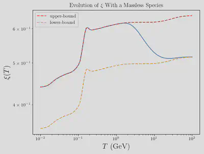
The senario in which there exists at least on massless species is a bit simpler than the case of all massive species. This is because the lower bound on $\xi^3h_{d}$ is much simpler. In this case, the bounds on $\xi$ are: $$\begin{align} \left(h(T)\dfrac{h_{d}(T_{d,\infty})}{h(T_{\infty}) \sum_{i}\eta_{i}g_{i}}\right)^{1/3}\xi_{\infty} < \xi < \left(h(T)\dfrac{h_{d}(T_{d,\infty})}{h(T_{\infty}) g_{\ell}}\right)^{1/3}\xi_{\infty} \end{align}$$ Here we’ve take $g_{\ell}$ to be one of the massless species. If we have many massless species, we can strengthen the lower bound by replacing $g_{\ell}$ with a sum over all massles species. Let’s modify our previous model by adding in a massless particle.
function dark_dof_entropy(model::ToyModel)
  hη = dof_entropy(model.η)
  hΔ = dof_entropy(model.Δ)
  h::Float64 = isfinite(hη) ? hη : 0.0
  h += isfinite(hΔ) ? hΔ : 0.0
  h += 2.0 # massles vector boson
  h
end

function ξ_lower_bound(T::Float64, model::ToyModel)
  model.sm.T = T
  hsm::Float64 = dof_entropy(model.sm)
  hsminf::Float64 = 106.83
  hdinf::Float64 = 7.0 / 8.0 * 4model.N + 2.0 * (model.N^2 - 1) + 2.0;
  ξinf::Float64 = 1.0
  sumg::Float64 = model.η.g + model.Δ.g * 7/8 + 2.0
  cbrt(hsm * hdinf * ξinf^3 / (hsminf * sumg))
end

function ξ_upper_bound(T::Float64, model::ToyModel)
  model.sm.T = T
  hsm::Float64 = dof_entropy(model.sm)
  hsminf::Float64 = 106.83
  hdinf::Float64 = 7.0 / 8.0 * 4model.N + 2.0 * (model.N^2 - 1) + 2.0;
  ξinf::Float64 = 1.0
  sumg::Float64 = 2.0
  cbrt(hsm * hdinf * ξinf^3 / (hsminf * sumg))
end

function compute_ξ(T::Float64, model::ToyModel)
  model.sm.T = T
  hsm::Float64 = dof_entropy(model.sm)
  hsminf::Float64 = 106.83
  hdinf::Float64 = 7/8 * 4model.N + 2.0 * (model.N^2 - 1) + 2.0
  ξinf::Float64 = 1.0
  function residual(ξ::Float64)
    model.η.T = ξ * T
    model.Δ.T = ξ * T
    res::Float64 = dark_dof_entropy(model)*ξ^3 -hsm*hdinf*ξinf^3/hsminf
    return res
  end
  lb::Float64 = ξ_lower_bound(T, model)
  ub::Float64 = ξ_upper_bound(T, model)

  ξsol::Float64 = find_zero(residual, (lb*0.99, ub*1.01), Bisection())
  model.ξ = ξsol
  ξsol
end
Now let’s plot:
import PyPlot; const plt = PyPlot # python plotting
using LaTeXStrings

model = ToyModel(10.0, 1.0)

Ts = 10 .^(range(-2, stop=2.0, length=100))
ξs = [compute_ξ(T, model) for T in Ts]
ξs_ub = [ξ_upper_bound(T, model) for T in Ts]
ξs_lb = [ξ_lower_bound(T, model) for T in Ts]

plt.figure(dpi=100)
plt.title(L"Evolution of $\xi$ With a Massless Species")
plt.plot(Ts, ξs)
plt.plot(Ts, ξs_ub, "--", label="upper-bound")
plt.plot(Ts, ξs_lb, "--", label="lower-bound")
plt.yscale("log")
plt.xscale("log")
plt.xlabel(L"$T \ (\mathrm{GeV})$", fontsize=16)
plt.ylabel(L"$\xi(T)$", fontsize=16)
plt.legend()
plt.gcf()

The behavior that we are seeing shouldn’t be too surprising. Our bounding curves for $\xi$ are both proportional to $h(T)$. Therefore, $\xi$ simply interpolates bewteen to different scalings of $h(T)$.
Case 3: SM Temperature from the Dark Temperature
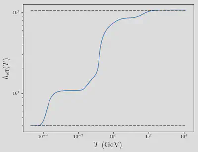
Suppose we want to compute the tempertature of the SM in given the a dark sector temperature. Then, we need to solve the following equation: $$\begin{align} \xi^3(T_{d}) = \dfrac{T_{d}^3}{T^3} = \dfrac{h(T)}{h_{d}(T_{d})}C_{\infty} \end{align}$$ In this case, one should think of $T_{d}$ as a fixed number and $T$ being a function of $T_{d}$. Isolating the constant pieces, we find: $$\begin{align} h(T)T^3 = \dfrac{T_{d}^3h_{d}(T_{d})}{C_{\infty}} \end{align}$$ The LHS of this equation is constant. Let’s look at a plot $h(T)$ for the SM.
using DelimitedFiles
import PyPlot; const plt = PyPlot # python plotting
using LaTeXStrings

sm_data = readdlm(string(@__DIR__) * "assets/data/smdof.csv", ',', skipstart=1)
sm_data_ts = sm_data[:, 1];
sm_data_hs = sm_data[:, 3];

plt.figure(dpi=100)
plt.plot(sm_data_ts, sm_data_hs)
plt.plot(sm_data_ts, [sm_data_hs[end] for _ in 1:length(sm_data_ts)], "k--")
plt.plot(sm_data_ts, [sm_data_hs[1] for _ in 1:length(sm_data_ts)], "k--")
plt.yscale("log")
plt.xscale("log")
plt.ylabel(L"$h_{\mathrm{eff}}(T)$", fontsize=16)
plt.xlabel(L"$T \ (\mathrm{GeV})$", fontsize=16)
plt.gcf()

From this plot, we can see that $h(T)$ is bounded from above and below. The bounding values are: $$\begin{align} h_{\mathrm{min}} \approx 3.93 < h(T) < 106.83 \approx h_{\mathrm{max}} \end{align}$$ It is therefore straight forward to find bounds on $T$: $$\begin{align} \dfrac{T_{d}^3h_{d}(T_{d})}{C_{\infty}h_{\mathrm{max}}} < T < \dfrac{T_{d}^3h_{d}(T_{d})}{C_{\infty}h_{\mathrm{min}}} \end{align}$$ Given these bounds, one can use a bisection method to solve for $T$ given a value for $T_{d}$.