Solving the Boltzmann Equation
Introduction
In this notebook, we will investigate how to solve the Boltzmann equation in order to determine the relic abundance of a species. Our focus will be on a species which represents a dark matter (DM) particle. We will assume that the dark matter interacts with the standard model (SM) through a massive mediator with interactions that look like $\bar{\chi}\chi\to \mathrm{SM}_{1} + \mathrm{SM}_{2}$, i.e. through a $2\to2$ interaction. For these types of interactions, the Boltzmann equation takes the form of: $$\begin{align} \dfrac{dn}{dt} + 3Hn = -\langle\sigma v\rangle(n^2 - n_{\mathrm{eq}}^2) \end{align}$$ where $n$ is the DM number density, $n_{\mathrm{eq}}$ is the DM equilibrium number density, $H$ is the hubble constant and $\langle\sigma v\rangle$ is the annihilation cross section for DM into SM particles. As is, this equation is in poor form. We will make several changes to bring it into a more suitible form for numerically solving.
Our first change will be to define the so called comoving number density, $Y$. This will be defined as: $$\begin{align} Y = \dfrac{n}{s} \end{align}$$ where $s$ is the SM entropy density. Note that the total SM entropy is conserved, i.e. $a^3s = \mathrm{constant}$ with $a$ being the scale factor of the universe. This implies that: $$\begin{align} \dfrac{d}{dt}a^3s = 3\dfrac{da}{dt}a^2s + a^3\dfrac{ds}{dt} = 0 \end{align}$$ If we rearange this equation and recall that $d\log(a)/dt = H$, we find that: $$\begin{align} \dfrac{ds}{dt} = -3\dfrac{1}{a}\dfrac{da}{dt}s = -3Hs \end{align}$$ This relation will allow us to determine $dY/dt$: $$\begin{align} \dfrac{1}{s}\dfrac{dn}{dt} &= \dfrac{dY}{dt} - 3HY \end{align}$$ Therefore, the Boltzmann equation for $Y$ is: $$\begin{align} \dfrac{dY}{dt} = -s\langle\sigma v\rangle(Y^2 - Y_{\mathrm{eq}}^2) \end{align}$$ where we defined $Y_{\mathrm{eq}} = n_{\mathrm{eq}}/s$. Next, we will change independent variables from time to temperature. To do this, we again us $\dot{s}/s = -3H$. Using the explict form $s=2\pi^2/45 hT^3$ ($h$ being the number of d.o.f. in entropy), one finds that: $$\begin{align} -3H = \dfrac{1}{s}\dfrac{ds}{dt} = \dfrac{3}{T}\left(1 + \dfrac{T}{3h}\dfrac{dh}{dT}\right) \dfrac{dT}{dt} \end{align}$$ Therefore, $$\begin{align} \dfrac{dt}{dT} =-\dfrac{1}{HT}\left(1 + \dfrac{T}{3h}\dfrac{dh}{dT}\right) \end{align}$$ We can use this relationship to determine $dY/dT$: $$\begin{align} \dfrac{dY}{dT} = \dfrac{dt}{dT}\dfrac{dY}{dt} = \dfrac{s}{HT}\left(1 + \dfrac{T}{3h}\dfrac{dh}{dT}\right) \langle\sigma v\rangle(Y^2 - Y_{\mathrm{eq}}^2) \end{align}$$ Another change people usually make is again changing the indepednent variable from $T\to x = m/T$ where $m$ is the mass of the DM particle. If we make this change, we find that: $$\begin{align} \dfrac{dY}{dx} =- \dfrac{s}{Hx}\left(1 + \dfrac{T}{3h}\dfrac{dh}{dT}\right) \langle\sigma v\rangle(Y^2 - Y_{\mathrm{eq}}^2) \end{align}$$ We can expand out the definitions of $s$ and $H=\sqrt{8\pi\rho/3}/M_{\mathrm{pl}}$ $$\begin{align} H = \sqrt{\dfrac{8\pi G}{3}\rho} = \sqrt{\dfrac{8\pi^3}{90}}\sqrt{g}\dfrac{T^2}{M_{\mathrm{pl}}} \end{align}$$ to obtain: $$\begin{align} \boxed{\dfrac{dY}{dx} =- \sqrt{\dfrac{\pi}{45}}\dfrac{m M_{\mathrm{pl}}}{x^2}g^{1/2}_{\star} \langle\sigma v\rangle(Y^2 - Y_{\mathrm{eq}}^2)} \end{align}$$ where we defined: $$\begin{align} g^{1/2}_{\star} \equiv \left(1 + \dfrac{T}{3h}\dfrac{dh}{dT}\right) \dfrac{h}{\sqrt{g}} \end{align}$$ This is typically how people quote the Boltzmann equation. However, one final set of modifications needs to be made for numerical purposes. $Y$ can vary over many orders of magnitude. Thus, it is very useful to define $W\equiv\log(Y)$. Then, $W$ only undergoes order $1$ changes. Additionally, it is useful to work with the $\log(x)$ instead of $x$. Making these changes we find that: $$\begin{align} \boxed{\dfrac{dW}{d\log(x)} =- \sqrt{\dfrac{\pi}{45}}\dfrac{m M_{\mathrm{pl}}}{x}g^{1/2}_{\star} \langle\sigma v\rangle(e^{W} - e^{2W_{\mathrm{eq}}-W})} \end{align}$$ In the next sections, we will solve this equation.
Simple Model
In many cases, the thermally averaged annihilation cross section can be brought into the form: $$\begin{align} \langle\sigma v\rangle = \langle\sigma v\rangle_{0}x^{-n} + \mathrm{O}(x^{-n-1}) \end{align}$$ In this form, we can simplify the Boltzmann equation to: $$\begin{align} \dfrac{dW}{d\log(x)} =- \sqrt{\dfrac{\pi}{45}}\dfrac{m M_{\mathrm{pl}}}{x^{n+1}}g^{1/2}_{\star} \langle\sigma v\rangle_{0}(e^{W} - e^{2W_{\mathrm{eq}}-W}) \end{align}$$
Evolution of $W = \log(n/s)$
Now, let’s define a model:
using DarkSUN

mutable struct DarkMatterModel
  χ::ThermodynamicFermion
  n::Int64
  sm::StandardModel
  σ0::Float64
end

"""
  DarkMatterModel(m::Float64, n::Int64, σ0::Float64)

Default constructor for DM model

# Arguments
- `m::Float64`: DM mass
- `n::Int64`: interaction order - 0: s-wave, 1: p-wave and so on.
- `σ0::Float64`: thermal cross section coefficient
"""
function DarkMatterModel(m::Float64, n::Int64, σ0::Float64)
  χ = ThermodynamicFermion(m, 2.0)
  DarkMatterModel(χ, n, StandardModel(), σ0)
end;
To solve the Boltzmann equation, we will use DifferentialEquantions.jl
(for solving the differential equation) and DarkSUN (for thermal functions
such as $g^{1/2}_{\star}$ and $n_{\mathrm{eq}}$.) Let’s define the Boltzmann
equation:
using DifferentialEquations

const Mpl = 1.220910e19

"""
  boltzmann(w, p, logx)

Boltzmann equation in `DifferentialEquations.jl` format.

# Arguments
- `dW::Array{Float64, 1}`: derivative of log of number density over SM entropy density
- `W::Array{Float64, 1}`: log of number density over SM entropy density
- `model::DarkMatterModel`: model
- `logx::Float64`: log of mass over temperature
"""
function boltzmann!(dW::Array{Float64, 1}, W::Array{Float64, 1},
                   model::DarkMatterModel, logx::Float64)
  x::Float64 = exp(logx)
  # update the temperature
  model.χ.T = model.χ.mass / x
  model.sm.T = model.χ.mass / x
  pf::Float64 = (-sqrt(π/45) * model.σ0 * model.χ.mass * Mpl * sqrt_gstar(model.sm) / x^(model.n+1))
  Weq::Float64 = log_neq(model.χ) - log_entropy_density(model.sm)
  dW[1] = pf * (exp(W[1]) - exp(2Weq - W[1]))
end


"""
  jacobian(w, p, logx)

Jacobian of the boltzmann equation in `DifferentialEquations.jl` format.

# Arguments
- `J::Array{Float64, 2}`: derivative of log of number density over SM entropy density
- `W::Array{Float64, 1}`: log of number density over SM entropy density
- `model::DarkMatterModel`: model
- `logx::Float64`: log of mass over temperature
"""
function jacobian!(J::Array{Float64, 2}, W::Array{Float64, 1},
                   model::DarkMatterModel, logx::Float64)
  x::Float64 = exp(logx)
  # update the temperature
  model.χ.T = model.χ.mass / x
  model.sm.T = model.χ.mass / x
  pf::Float64 = (-sqrt(π/45) * model.σ0 * model.χ.mass * Mpl * sqrt_gstar(model.sm) / x^(model.n+1))
  Weq::Float64 = log_neq(model.χ) - log_entropy_density(model.sm)
  J[1,1] = pf * (exp(W[1]) + exp(2Weq - W[1]))
end;

"""
  solve(model, logxspan)

Solve the Boltzmann equation for the given model.

# Arguments
- `model::DarkMatterModel`: DM model
- `logxspan::Tuple{Float64}`: range of log(x)
"""
function solve!(model::DarkMatterModel, logxspan::Tuple{Float64, Float64})
  # Initialize temperatures
  model.χ.T = model.χ.mass * exp(-logxspan[1])
  model.sm.T = model.χ.mass * exp(-logxspan[1])
  # Initial value for W
  W0 = log_neq(model.χ) - log_entropy_density(model.sm)
  # Create ODE problem
  ff = ODEFunction(boltzmann!;jac=jacobian!)
  prob = ODEProblem(ff,[W0],logxspan, model)
  # Solve it!
  solve(prob, Rodas5(autodiff=false));
end
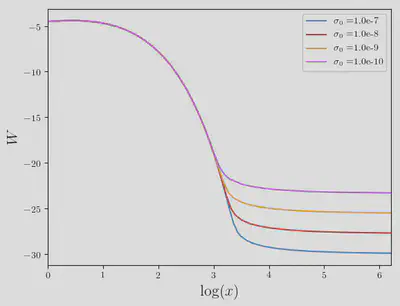
Now let’s solve for various values of $\sigma_{0}$
# Values for logx
logxspan = (log(1), log(500))
σ0s = [1e-7, 1e-8, 1e-9, 1e-10]
models = [DarkMatterModel(100.0, 0, σ0) for σ0 in σ0s]
sols = [solve!(model, logxspan) for model in models];
Now we can plot the solution:
import PyPlot; const plt = PyPlot # python plotting
using LaTeXStrings

plt.figure(dpi=100)
for (i, sol) in enumerate(sols)
  plt.plot(sol.t, sol[1,:], label=L"$\sigma_{0} = $"*string(σ0s[i]))
end
plt.ylabel(L"$W$", fontsize=16)
plt.xlabel(L"$\log(x)$", fontsize=16)
plt.xlim([logxspan[1], logxspan[2]])
plt.legend()
plt.gcf()

Relic Densities
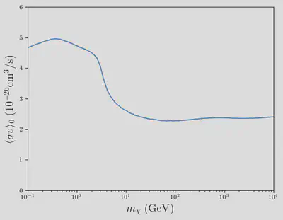
Recall that the relic density is computed using: $$\begin{align} \Omega_{\chi} h^2 = \dfrac{s_{0}}{\rho_{c}}m_{\chi}Y(x=\infty) \end{align}$$ where $s_{0} = 2891.2 \mathrm{cm}^{-3}$ and $\rho_{c} =1.05375\times10^{-5}\mathrm{h}^2\mathrm{GeV}\mathrm{cm}^{-3}$. Let’s perform the excercise of computing the relic density for values values of $m_{\chi}$ and $\langle\sigma v\rangle_{0}$. We will then plot the contours for which the combination $(m_{\chi}, \langle\sigma v\rangle_{0})$ gives the correct observed relic density, which is $\Omega_{\chi}h^2=0.1198$. First, let’s write a function to solve the Boltzmann equantion and compute the relic density:
const ρc = 1.05375e-5
const s₀ = 2891.2

function relic_density(model::DarkMatterModel)
  sol = solve!(model, (log(1), log(1000)))
  s₀ / ρc * model.χ.mass * exp(sol[1, end])
end;
Now, let’s compute the relic density for DM masses between $10$ and $10^4\mathrm{GeV}$ with cross sections between $10^{-12}$ and $10^{-7} \mathrm{GeV}^{-2}$.
mχs = 10 .^(range(-1, stop=4, length=150))
σ0s = 10 .^(range(-12, stop=-7, length=150))
models = [DarkMatterModel(mχ, 0, σ0) for mχ in mχs, σ0 in σ0s]
Ωh²s = [relic_density(model) for model in models];
Now, let’s plot the contours of correct relic density:
using Contour
const Ωh²cdm = 0.1198

cs = contour(mχs, σ0s, Ωh²s, Ωh²cdm)

plt.figure(dpi=100)
for line in lines(cs)
  xs, ys = coordinates(line)
  plt.plot(xs, ys .* 1.16733e-17 * 1e26) # convert units to 10^-26 cm^3/s
end
plt.xscale("log")
plt.ylabel(L"$\langle\sigma v\rangle_{0} \ (10^{-26}\mathrm{cm}^{3}/\mathrm{s})$", fontsize=16)
plt.xlabel(L"$m_{\chi} \ (\mathrm{GeV})$", fontsize=16)
plt.ylim([0, 6])
plt.xlim([minimum(mχs),maximum(mχs)])
plt.gcf()
